Linear Models
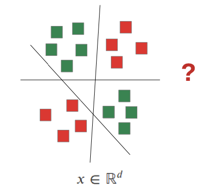
Recall Classification:
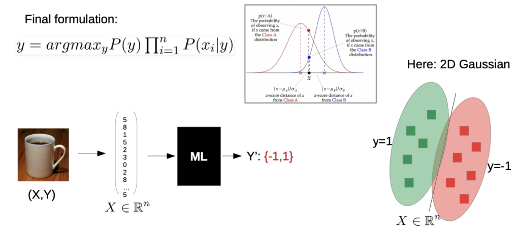
→ there are other possibilities than Gaussian, e.g. geometrically
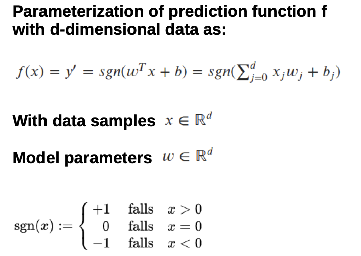
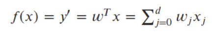
Parameterization
e.g. straight line (linear, 2D)
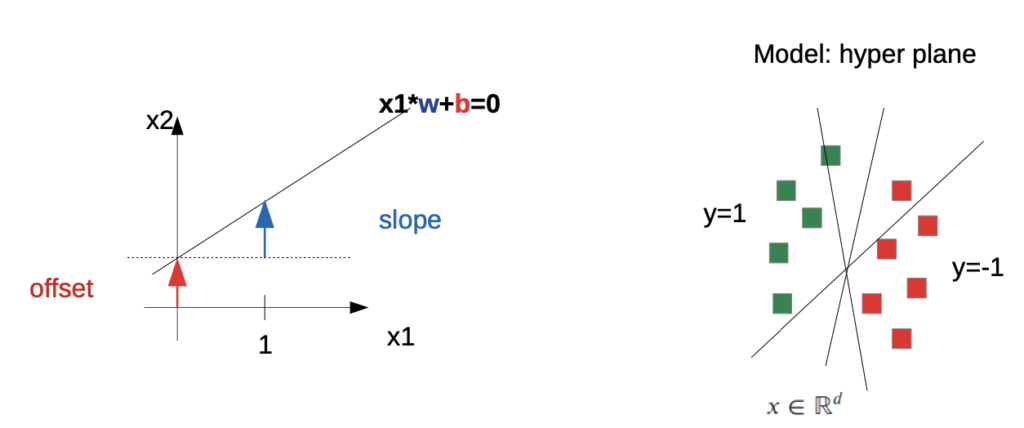
How to find the Parameters?
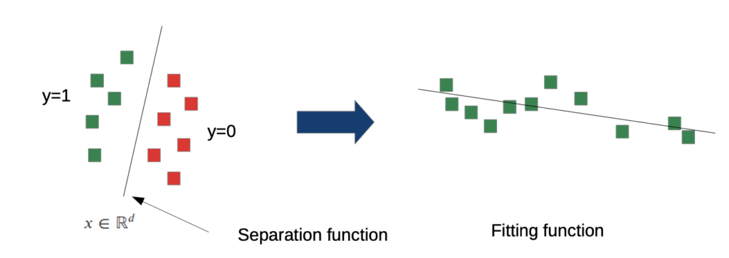
→ we “draw” a line between the examples
→ many optimization methods to get better parameters
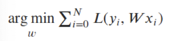
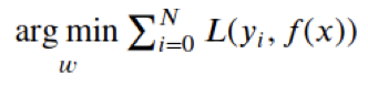
Minimize the error (the Loss function L):
- Loss function has to be differential
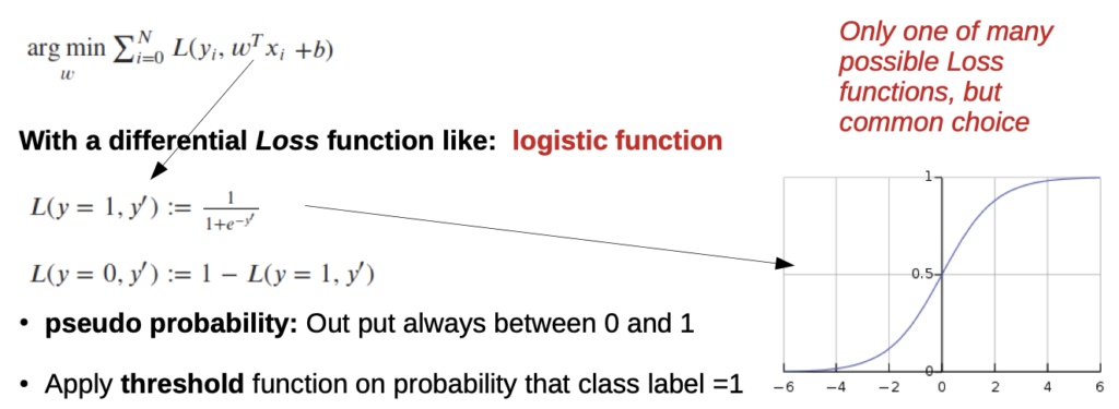
- logistic function: Values between 0 and 1 (pseudo probability)
two parameters, many possible solutions
→ solution in vector spaces

- each point is a possible solution
- we can compute the gradient at each point, the direction of the gradient to the parameters with minimal errors
→ Gradient Descent ALgorithm
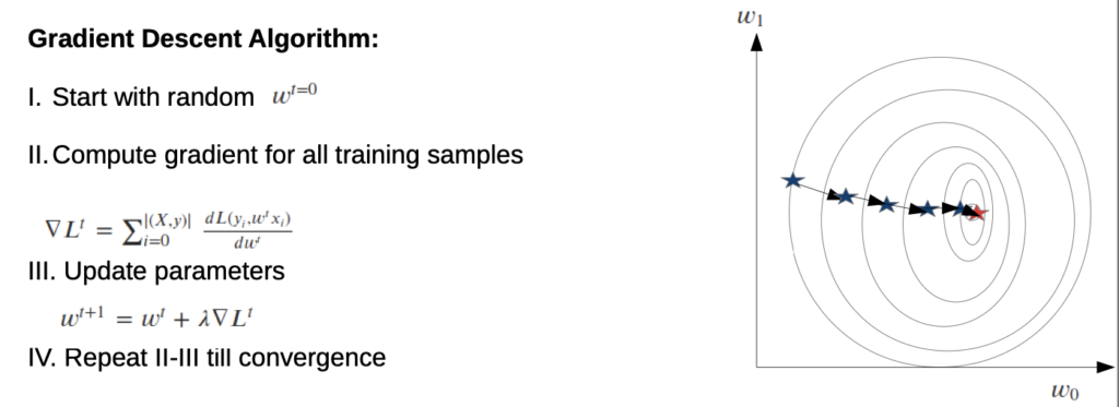
Lamda (Step 3) is the step size or learning rate, usually quite small scalar like 0.001
- with a higher step size, we get a faster solution, but may be less accurate
! pay attention if the algorithm is convex, otherwise a local minima could be calculated!
How long to repeat?
Different possibilities:
- pre set number of iterations
- loss limit
- loss not changing

Summary:
- Parameterization
- Define Loss function
- Optimize Parameters until satisfaction
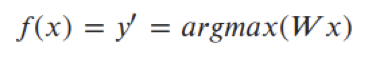
Multi class problems
→ one vector per class, summarized to matrix
Optimization problem is almost the same:
Change Loss to SOFTMAX function to normalize sum aver all probabilities to one:

Use “one-hot” coding of y
- instead of giving a single probability, give a probability for each class
- Loss function returns now a vector
Different possibilities:
- one non-linear, complex function
- multiple linear functions (ensemble learning)
Ensemble Learning (Random Forests)
- many weak models decide together (by voting)
- Easy to implement and to parallelize
- Does not tend to overfit
- Build in Feature-Selection→ doesn’t only show us what is chased, but also why
Decision Trees
- base classifier for Random Forests
- normally, decision trees aren’t good, because they tend to simply memorize decisions→ recombination from different forests
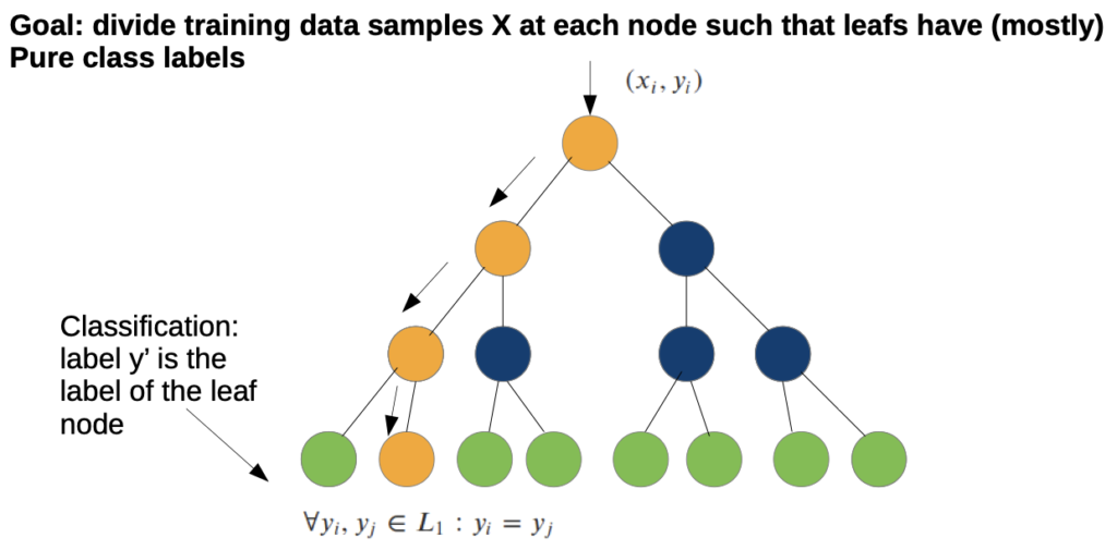
- we need a splitting function that will produce (almost) pure class labels
Top Down Training:
Assume k classes and data of dimension d
Fill tree with ALL training samples from the root down In each node: compute probability for all class labels in node n
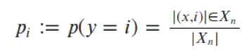
Compute node purity based on class probabilities
Node purity: How clear is the node if it would be the last one
Split node along one dimension such that purity of children is increasing (optimization)
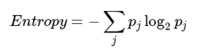
Entropy (a way to measure impurity):
Gini index:

…
Split optimization (Simple Line search) examples
…
But we train multiple trees with the same data, how to avoid memorization?
we get randomness from:
- we select random variables→ trees are not the same
- Bootstrapping data→ not every tree gets the same data
Regression
not every prediction is discrete (Class X, Class Y, …)
→ some are continuous (like costs in a taxi)
→ fitting function instead of separation function
You can still use the same framework:
Simply need new loss function in the optimization

Measurements
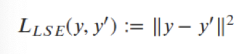
- least square error:
- many other measures possible, e.g. L1 (Histogram intersection)
Regression with Random Forests:

we need a new splitting function (we don’t have purity)
→ goal: reduce “data spread” in node
→ use simple statistical measure like “mean square error”
Non-linear models I
Need for non-linear models
Linear models are very limited, for example the “X-Or” Problem
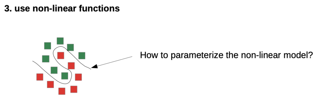
How to add non-linearity?
Three canonical ways:
- extracting non-linear features (already learned)
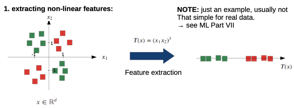

Add non-linearity to our simple classifier
Step 1: add a simple element-wise non-linear mapping

the non-linear mapping can be anything which can be done to every element, like square, root, …
What are good choices for these functions?
- Properties
- between 0 and 1 → pseudo probability interpretation
- stable range of output → gradient optimization
- Common choices
- Sigmoid function
- Tanh
- …
Step 2: concatenate several of these operations
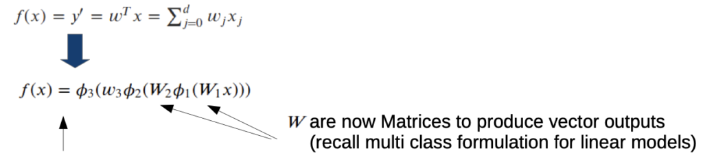
→ we combine several transformations:
X → Matrix/Vector Mult operation → Element wise non-linear operation → Matrix/Vector Mult operation …….. → f (x)
Note: if the W is large enough, we theoretical need only two concatenations to approximate any smooth function
Then we need a Loss-function
problem didn’t change
→ same approach as in the linear case
- the parameters are set in W (Matrix/Vector Mult operation)
- non-linear operations are preset, they don’t have to change
→ optimization problem is the same as by linear
Problem: Overfitting
prevent already during optimization problem
→ adding regularization to the Loss function
L2 regularization:

- all parameters to be learned in square
- Lambda (Scalar hyper parameter) sets how strong complexity is “punished”
L1 regularization:
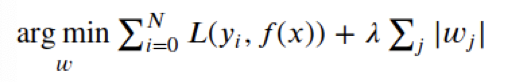
→ Regularization will punish higher parameter values
→ smoother model
→ training errors allowed
Neuronal Networks
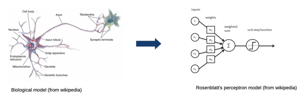
- inputs from other neurons
- every input has a (learnable) weight→ the more the input is activated, the stronger is the connection
- weighted sum is a neuron with sums up all incoming signals with their weights and gives it to a non-linear function which decides if the sum is big enough to “fire” (signalling)→ if yes, signal goes to the other neurons
Comparison to our previous non-linear model
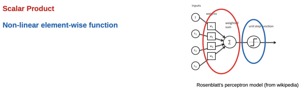
- Inputs are our X
- Input = 1 is our constant offset (our b in Wx + b)
Connect multiple neurons
A simple Neuronal Network:

- our w turns into W
A deeper (fully connected) Neuronal Network
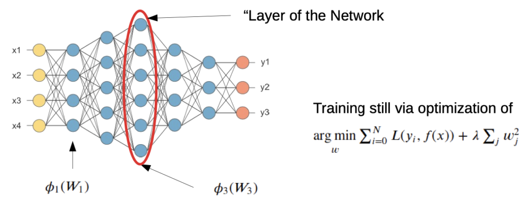
- multiple Layers (5 Layers in this example)
- “fully connected” means all outputs of a layer are connected to all coming layers
Code Exercises
(Link to Github)