Feature Extraction and Deep Learning
Feature Extraction
Recall Supervised Classification
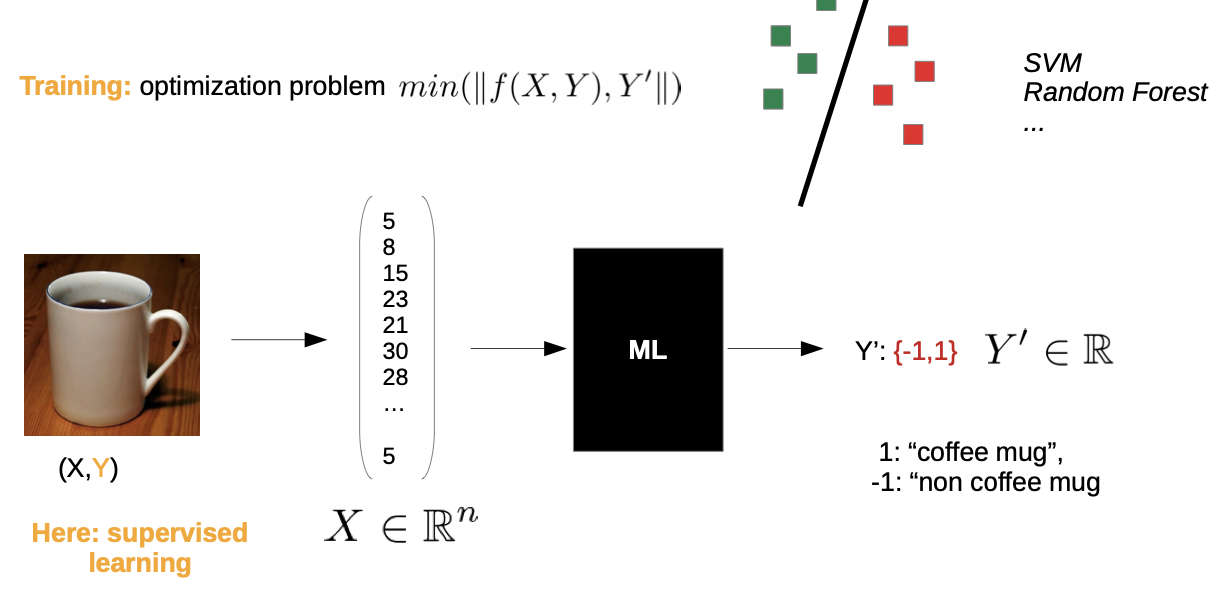
- the chosen vector space representation aligns the chosen model and how we make a classification
- earlier, we took pixel by pixel and write it in the vector space

Problem: If we took a slightly other camera angle, there is still a coffee mug, but it’s a whole different point in the space
→ Classification could be wrong
Different solutions:
- if we have a picture of every possible camera angle, we could evaluate more correctly → what if the size of the coffee mug differs?
- feature engineering “preparation”, so our model can evaluate correctly
Feature Engineering
Solution: Shallow Learning
Unstructured data —> Feature Engineering (mathematical operator) —> “mathematical finger print” (feature space)
Properties:
- preserves information semantic classes have in common, throws away the rest
- the mathematical finger print doesn’t change much when e.g. the camera angle varies (called invariant or robust)
- Reduces the dimensionality of the problem
Drawbacks:
- good feature extraction is hard to find (high manual workload)
- feature extraction is very data specific
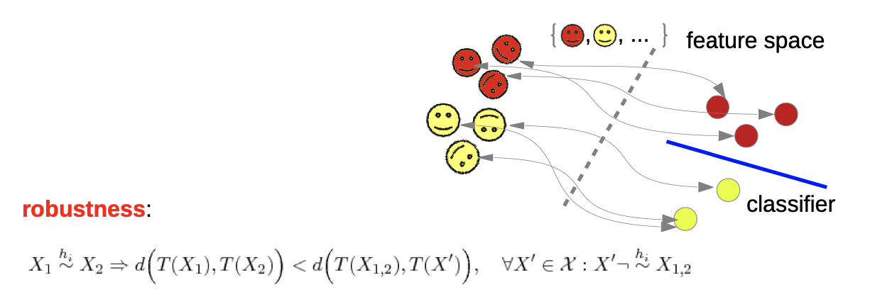
Invariant Theory
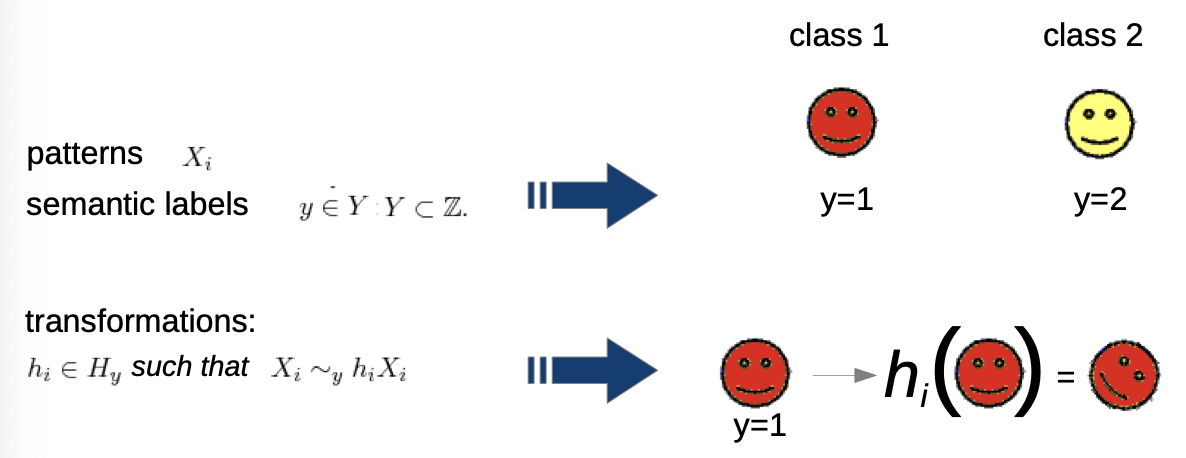
- transformations can be anything, even don’t have to be mathematically
→ we want to define invariance:
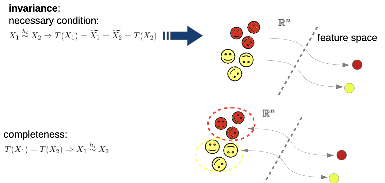
- given are two data points that are equivalent under transformation
- feature extraction T
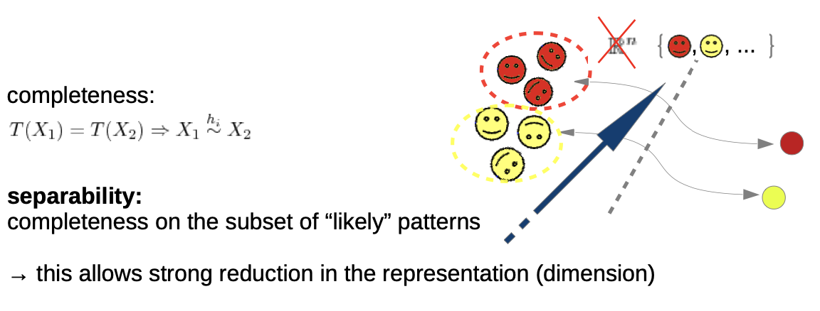
- we need completeness (transformation backwards), otherwise the trivial solution T(x) = 0 would be valid (we don’t need to know how “much” they were transformed, but which class they are assign)
→ in praxis, these is nearly impossible to reach
→ we “weaken” the invariance
separability: we don’t demand invariance for all, but for our training samples
Discussion
Feature extraction vs learning algorithms:
I. if we had perfect features, learning would be trivial
II. if we had perfect classifiers, we would not need features
Features are usually used to introduce prior knowledge about the structure of the data and variances to the learning algorithm.
There isn’t the perfect feature, most often you need clustering of different approaches.
In practice:
- Good features are hard to find
- Often based on complex mathematical functions
- Depend on the application (domain knowledge needed!)
Generic Approaches:
Invariance by differentiation: set properties into relation / normalization
Invariance by integration: compute average properties
Motivation
- Very high dimensional representations require a lot of data to fill this huge space (curse of dimensionality)
- Danger of overfitting is higher if space is only sparsely sampled
→ We would like to “compress” our data (with steerable loss) to a lower dimensional representation
Feature Reduction: PCA Recall:
- Co-VarianceMatrix (Week3)
- EigenValueDecomposition (Week2)
Combining both concepts for dimension reduction via Principal Component Analysis (PCA)
Feature Reduction: PCA
PCA Algorithm in a nutshell
- Compute Co-Variance Matrix of the data
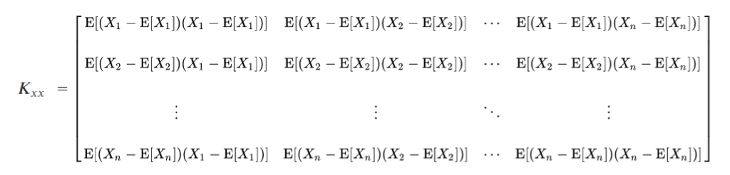
where E[X] is the expected value (mean)
- Compute Eigen Vectors and Values of K[xx]
- Sort Eigen Values
- Select cut-off value
- New basis: project to Eigen vectors New dimension: #Eigen values selected
Deep Learning
Intro
- On an implementational level, deep Learning are very large neuronal networks
- also called 3rd generation of neuronal networks
- we still are in machine Learning, there still isn’t a strong KI
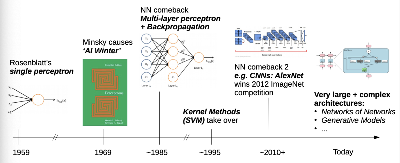
- Modern architectures have evolved very far from the original perceptron → in a pure Deep Learning lectures, we would go from left to right, but we focus on the modern models
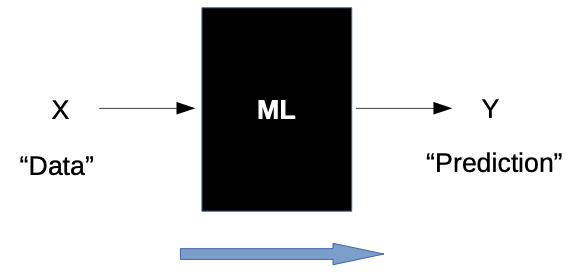
Deep Learning as a blackbox
- is a subset of ML algorithms
- our blackbox model is still valid
What is different?
Before:
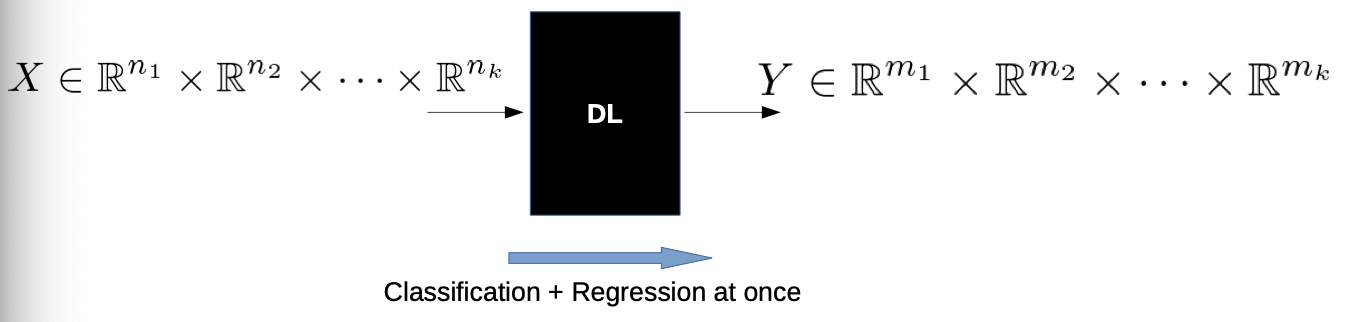
- most ML algorithms are limited to tight input/output domains e.g. image to vector, always scalar output
- Pre- and post-processing needed to solve more complex problems!
Now:
- capacity of learned mapping is better → natively allows structured (tensor) in- and output
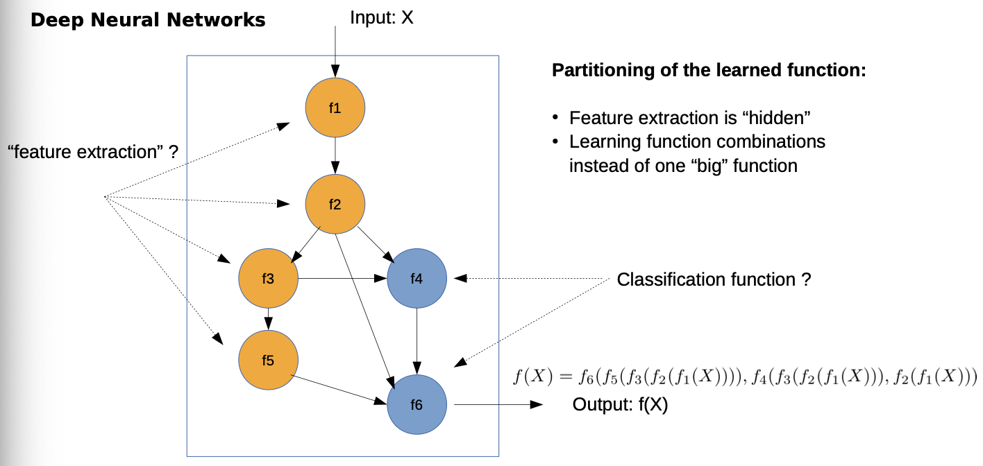
- “End to End” learning: Feature extraction is difficult, can we make this step learnable? (Shallow Learning) → but still 2 steps, even if these steps are connected → “End to End” learning, learn decision space and function in one optimization problem

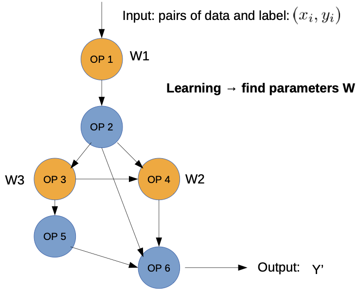
Opening the blackbox model
(brief intro)
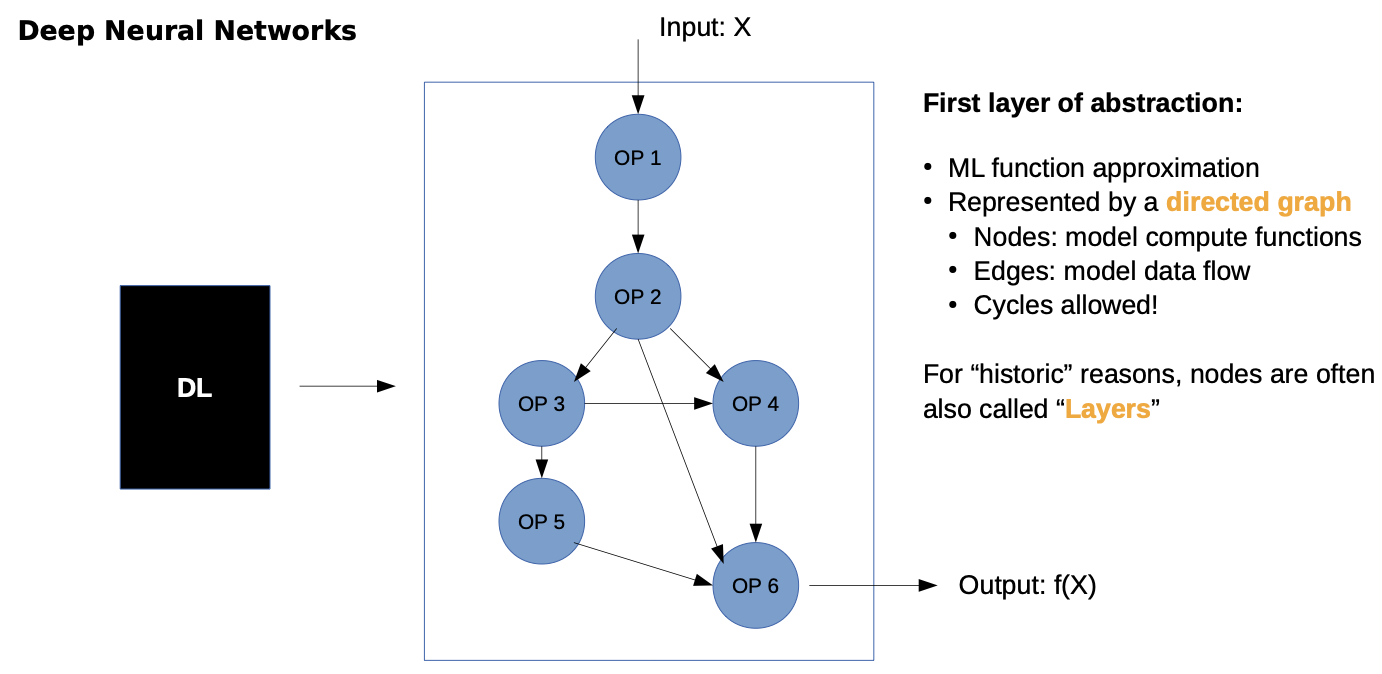
- we don’t have one big function, rather we partition the problem in other functions
- Only constraint: partially differentiable (for training)
- Depending on application and data some have learnable parameters, others are static
- In/Output are tensors
- later we can’t make this easy assignment, because steps are mixed
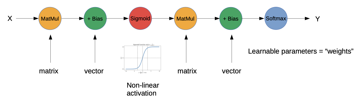
Simplest Example of DNN: Multi Layer Perceptron (MLP)
More complex deep DNN example:
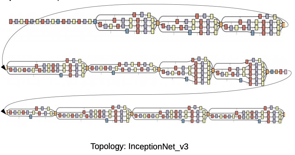
Training of Neural Networks
Training of DNNs is an optimization problem: (example for supervised learning)
1. Run data samples through graph → “forward feed”
2. Get result y’
3. Define differentiable “loss function” to measure “difference” between prediction and true label
4. Optimization objective: minimize loss
Optimization Problem:
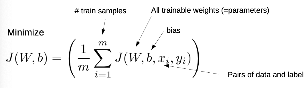
- J is our Loss function
Problem: Non CONVEX optimization problem in a very high dimensional space
→ we don’t know if the solution is the best one (could be local minima)
→ NP-HARD PROBLEM
→ numeric and stochastic solution
How to get the nested gradients?
→ With Back Propagation algorithm
- feed forward and compute activation
- compute error gradient between true Y and predicted Y’

- compute derivative by layer
→ chain rule (we calculate backwards each gradient with the chain rule)
- update all weights with small step in gradient direction
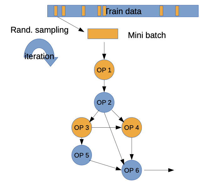
BUT: Using all of the training data to compute the gradient is computational infeasible
Instead: Monte Carlo approach: select random batch (small set of training data) per iteration to compute the gradient → SGD
Stochastic Gradient Descent (SGD)
we use random to escape from possible local minima and to calculate gradients without running over all data
→ non-smooth convergence
→ many iterations needed (also called epochs)
→ need additional parameters
- Step size (learning rate)
- Batch size
- …
Pitfalls of DNN training
- Optimization Algorithms have many hyper parameters (that have great effect on the outcome)
- Optimization is not deterministic (local minima, random initialization)
- Optimization is very compute intensive
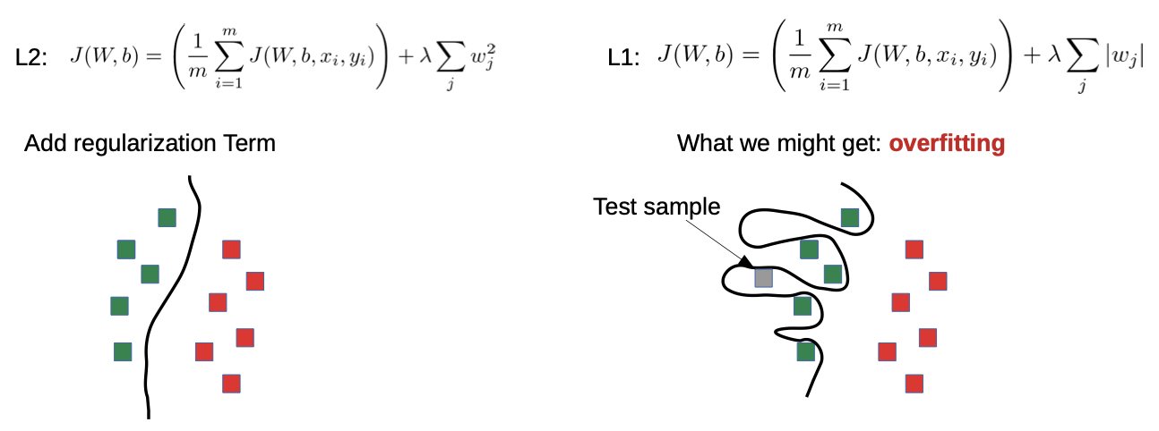
- DNN training is likely to overfit
→ regularization
- Needs a lot of training data to learn the underlying distributions
- not only many data points, also good sampling
- data annotation (for supervised DL)
→ especially in 3 to 5, progress in hardware and data are the core drivers
Basic Types of Deep Neuronal Network Architectures
Basic Architecture of Multi Layer Perceptron (2nd Generation Neuronal Networks):

Where are the Neurons?
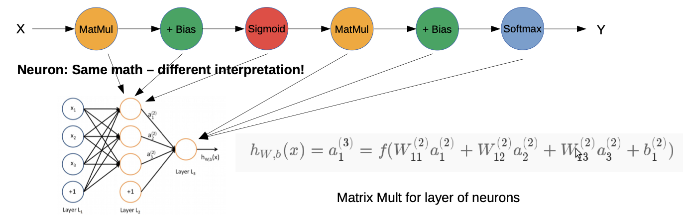
→ How do we implement the feature extraction?
→ we have to look at the operators
Convolutional Neuronal Networks (CNN)
- Most prominent type of DNN (LSTMs are catching up). Responsible for many practical breakthroughs
- Able to capture locality at multiple scales. Works well for data with locally embedded structures, e.g. images, videos, audio, graphs … even text
- Learns Filters which are applied via convolution (End-to-end optimization)
Typical Design: (AlexNet)
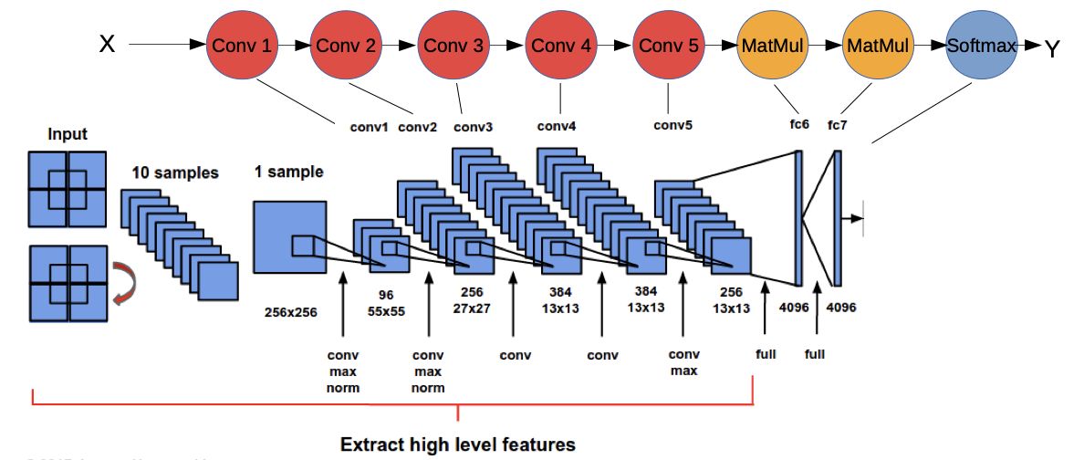
- New Conv operators
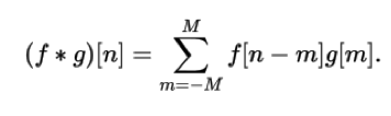
Exkurs: Convolution
- is a mathematical operation between two functions
(here over time series [t])

(wikipedia example animation here)
→ we have discrete functions, often multi dimensional, e.g. image in 2D
→ we have to adapt
Convolutional Filters
- f is the image
- g is the filter
- image is much larger than the filter
→ We “sum of an element-wise multiplication over a sliding window”
- = filter is moved over the image
Example:
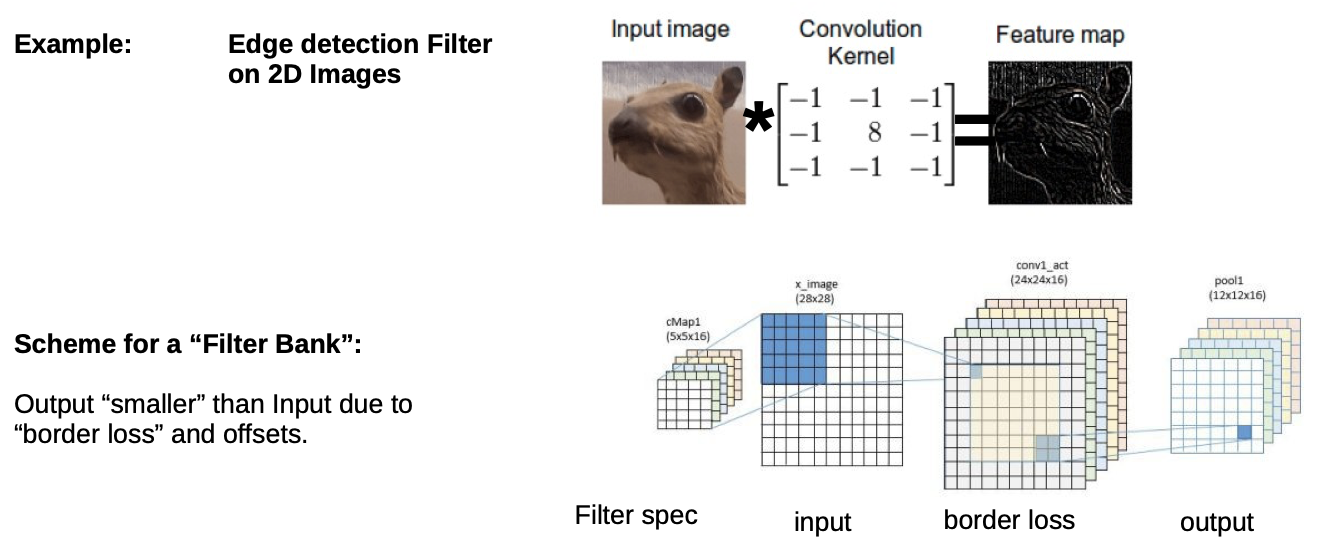
- we don’t select a filter (Convolution Kernel), we learn which filter fits best for our problem
- we have a “filter bank”, we choose which fits our problem the best
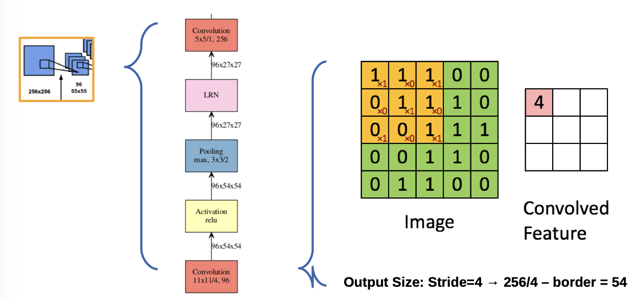
- Stride: step size in which we move
Capturing image statistics of natural scenes
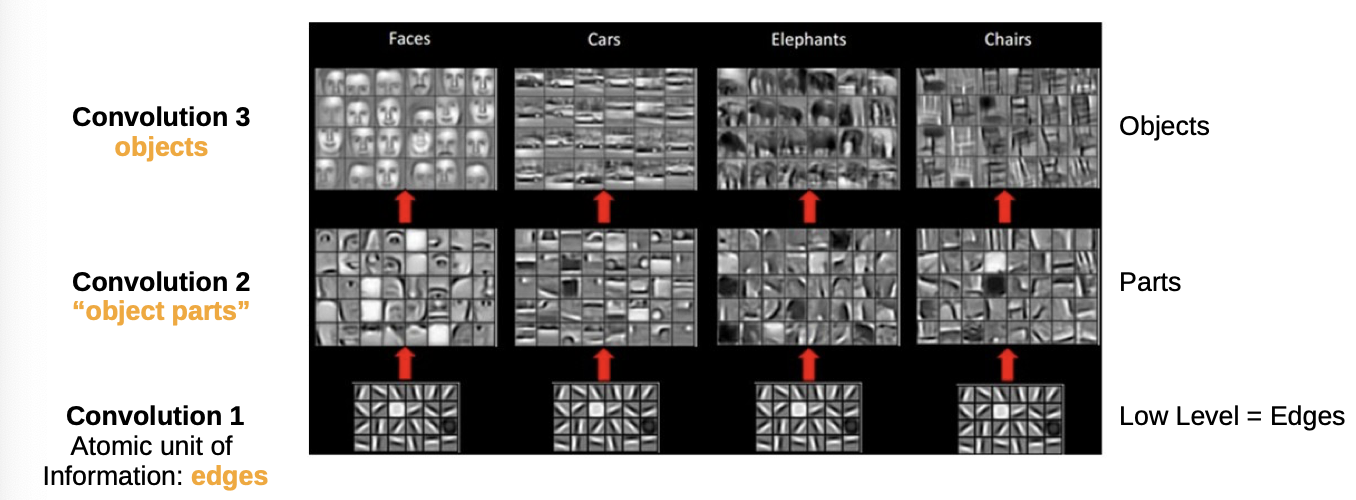
- at the lowest level, pictures are edges
Recurrent Neural Networks
- Networks for sequence learning
- typical applications: text analysis, translation (sequence to sequence), audio, sensor data → time series, well logs, …
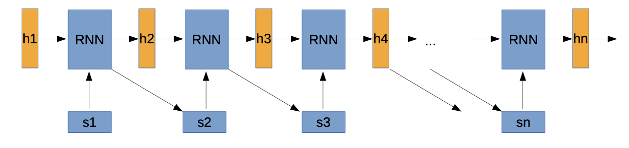
- s1, s2, … sn are Input sequence
- h1, h2, … hn are “hidden” vectors, coding the current state in the sequence → hn can be used, e.g. as input for classification
- Recurrent DNN, usually LSTM or GRU, but more complex DNN possible
- RNN predicts next sequence element
Generative Adversarial Neuronal Networks (GAN)
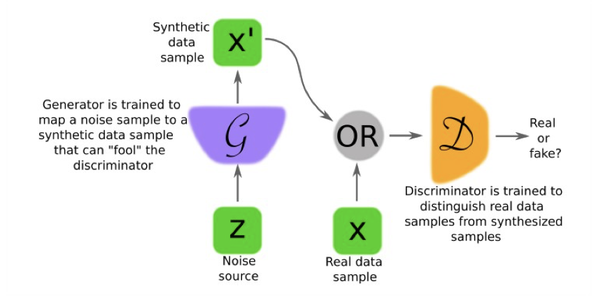
In a Nutshell, Generative Adversarial Nets are:
- No classification or Regression, instead we reproduce data (probabilities)
- Groups of DNNs (at least two)
- Working against each other → Generator gets a negative gradient if the Discriminator knows if the image was real or fake
- Min parts
- Discriminator Network
- Generator Network
Code Exercises
(Links to Github)