Linear Algebra and Quantum Mechanics
During my bachelors in mechanical engineering, I had a lot of math lectures. But I didn’t need to “update” the views I had about basic mathematical terms. I mostly continued the mathematical thinking which I still had from my A-levels. This changed when I started learning about Quantum Mechanics. I needed to question the previous knowledge I had, especially about linear algebra.
For my own clarification, I wanted to write the most important things down.
New Definition of Vectors
A vector is not simply an arrow in a coordinate system anymore; rather, a vector = an element / mathematical object that exists in a vector space.
Dirac Notation
The Dirac notation introduces the “ket” vector:
\[\vert\psi\rangle\]And its dual vector, the “bra”:
\[\langle\psi\vert\]The bra is also called the “hermitian” or “adjoint” of the original object.
The norm (length) of a vector:
\[\|\vert\psi\rangle\| = \sqrt{\langle\psi\vert\psi\rangle}\]I questioned the reason behind the Dirac Notation. But it turns out, it’s really helpful to prevent mistakes, especially when dealing with complex vectors.
What is a Vector Space?
A vector space V is a set of objects (vectors) over a field (real numbers, complex numbers, etc.) and has two binary operators:
- $\vert v\rangle + \vert u\rangle$ : vector addition
- result is also in vector space (closure)
- → vector spaces are closed under vector addition
- there are multiple vector addition axioms:
- commutativity
- associativity
- existence of an additive identity, also called zero vector
- 0 or $\vert \text{null}\rangle$ (not to be confused with $\vert 0\rangle$!)
- $\exists \vert \text{null}\rangle \in V$ such that
- $\vert v\rangle + \vert \text{null}\rangle = \vert v\rangle \forall \vert v\rangle \in V$
- existence of an additive inverse, which is just glorified subtraction. It means that for every vector in V, there is another vector in V, so that by addition it results in the 0 vector.
- $c \cdot \vert v\rangle$ : scalar multiplication
There are more axioms for vector addition and scalar multiplication but tbh, they are mostly self-explanatory. Here is a more complete list.
Also note that depending of the elements in a vector space, there are real vector spaces ⟷ complex vector spaces.
Spanning and Bases
This part is pretty straightforward, but it’s still important to define precisely.
Definition span: A set of vectors β = {v₁, v₂, …, vₙ} in a vector space V is called spanning, if every vector in V can be written as a linear combination of vectors in β. Such a set is said to span V.
Definition basis: A basis for a vector space V is a set of vectors β in V which is both linearly independent and spanning.
(Linear independent means that every vector within a set can’t be rebuilt using the others.)
Every vector $\vert v\rangle$ in a vector space V is a unique linear combination of the basis vectors.
For finite-dimensional vector spaces, the number of the vectors in a basis equals its dimension.
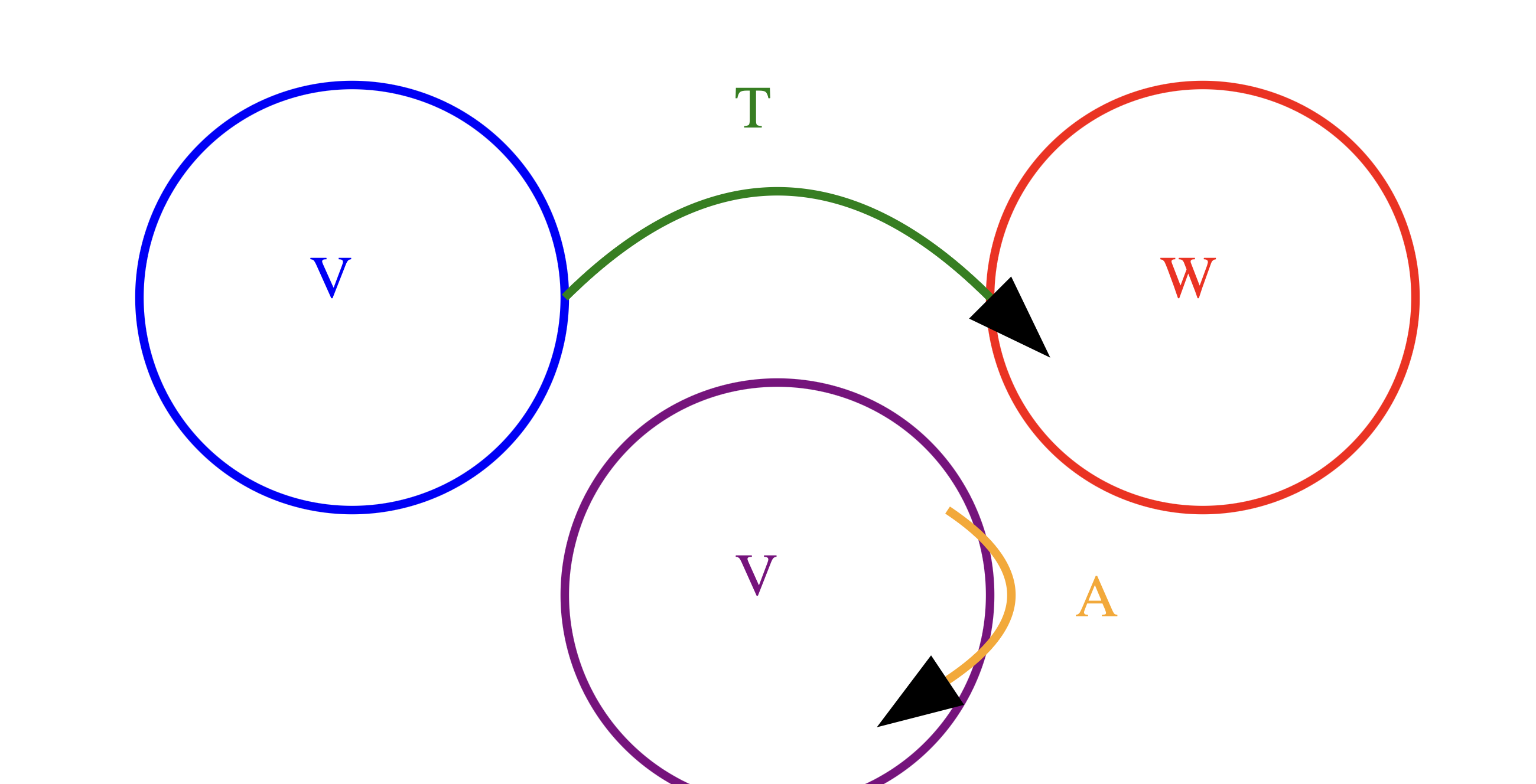
Linear Transformations
Definition: A linear transformation T from a vector space V to a vector space W (T : V → W) is a function that maps vectors from V to W while preserving the vector space structure.
Other important notes:
-
Difference injective ⟷ surjective: If the linear transformation doesn’t map one vector to multiple vectors, it’s injective. If every vector in the target space is mapped to, it’s surjective.
-
A linear transformation which can be undone by another linear transformation is called invertible, and the latter linear transformation is called the inverse of the former.
-
A linear operator A is a linear transformation from a vector space to itself.
Function ⟷ Linear Transformation
Functions
- A function is a general mapping from one set to another.
- It doesn’t necessarily preserve any algebraic structure.
- Can be non-linear.
Linear Transformations
- A specific type of function between vector spaces.
- Preserves vector addition and scalar multiplication.
- Always linear by definition.
Basically all linear transformations are functions, but not all functions are linear transformations.
Inner Product
An important example of a function is the inner product:
\[\left\langle \begin{pmatrix} c_1 \\ c_2 \\ \vdots \\ c_n \end{pmatrix}, \begin{pmatrix} d_1 \\ d_2 \\ \vdots \\ d_n \end{pmatrix} \right\rangle := \sum_{j=1}^{n} \overline{c_j} d_j\]Rules: (ψ, φ and χ = vectors, c = scalar)
- $\langle\psi,\phi+\chi\rangle = \langle\psi,\phi\rangle + \langle\psi,\chi\rangle$
- $\langle\psi, c \phi\rangle = c \langle\psi, \phi\rangle$
- $\langle\psi, \phi\rangle = \overline{\langle\phi, \psi\rangle}$ (“×” = complex conjugation)
- $\langle\psi, \psi\rangle$ is always real and non-negative and is zero only if ψ = 0
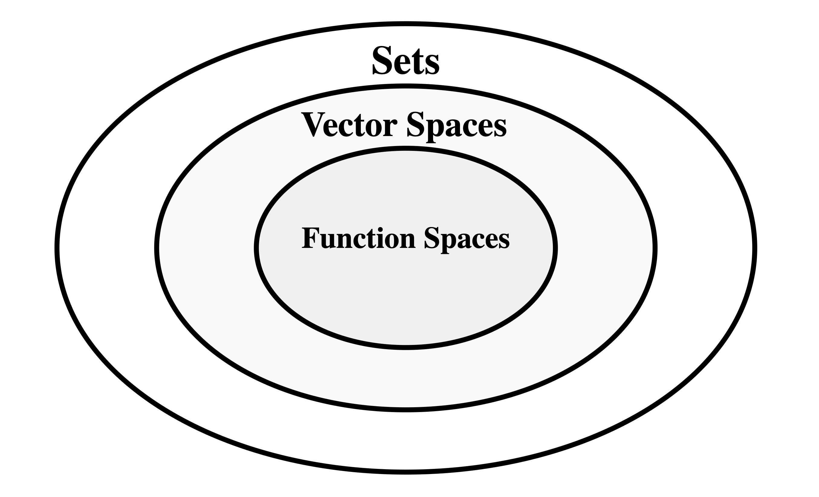
Sets, Vector Spaces, and Function Spaces
Now is also a good time to distinguish between a set, vector spaces and function spaces. Because by definition, a function space is actually a type of vector space.
Sets
A collection of objects with no inherent structure or operations defined. These elements could be anything, for examples: {1, 2, 3}, {apple, banana, cherry}, {x | x is a real number}.
Vector Spaces
A vector space is a set with additional structure and defined operations. It has to satisfy specific axioms related to vector addition and scalar multiplication. So all vector spaces are sets, but not all sets are vector spaces.
Function spaces
A function space is a set of functions that also has a vector space structure. The elements (functions) can be added and scaled, satisfying vector space axioms. So basically, function spaces = a certain type of vector spaces.
Hilbert Spaces
A Hilbert space is a vector space endowed with an inner product.
What does “endowed” mean?
I really struggled with this at first. “Endowed” in this context doesn’t refer to a two-step process. Being endowed with an inner product means that the inner product is a fundamental property of the space, not a separate calculation performed afterwards.
Vector representation in Hilbert Spaces
The keyword here is “representation”. The vector itself is not necessarily a nx1 matrix. Rather, it’s an abstract, mathematical object. There are two approaches how we can work with vectors:
1. Abstract Hilbert Space Approach
In this approach, we start with an abstract Hilbert space H. This space is defined by its properties rather than by specifying its elements explicitly (like I described, they are mathematical objects).
When we choose a basis {$\vert e_1\rangle$, $\vert e_2\rangle$, …, $\vert e_n\rangle$}, we can represent any vector $\vert\psi\rangle$ in H as a linear combination of these basis vectors:
\[\vert\psi\rangle = \sum_j c_j \vert e_j\rangle\]Here, the $c_j$ are complex numbers, but $\vert\psi\rangle$ itself is not identified with these numbers. Instead, there’s a correspondence between $\vert\psi\rangle$ and the collection of $c_j$.
This framework maintains a distinction between the abstract vector $\vert\psi\rangle$ and its representation in terms of components $(c_1, c_2, …, c_n)$. The basis can be changed easily without changing the vector itself.
2. Concrete Cn Approach
In this approach, we simply define H to be $\mathbb{C}^n$. Here, a vector $\vert\psi\rangle$ is directly identified with its components:
\[\vert\psi\rangle = (c_1, c_2, ..., c_n)\]In this case, there’s no distinction between the vector and its representation. The components $c_j$ are the vector.
When should we use what?
In practice, for finite-dimensional spaces, these approaches often lead to the same calculations. The difference is more in the interpretation and the conceptual framework.
For example, in the abstract approach, when you change basis, you’re representing the same abstract vector in a new way. In the $\mathbb{C}^n$ approach, changing basis looks more like a transformation of the vector itself.
The abstract approach is particularly useful when dealing with concepts like operators, where thinking about them as abstract entities acting on an abstract space can be more intuitive than thinking about them as matrices acting on columns of numbers.
In quantum mechanics, the abstract approach aligns well with the idea that quantum states have an existence independent of any particular measurement basis we might choose.
All around Eigen
To be continued…
Other Questions I Asked Myself
Can complex vectors be visualised?
I thought about a way to visualise complex vectors as a “mathematical object”. This turned out to be difficult to answer. Yes, for every complex element within a vector, you could add another axis, colour etc. There are several ways, as showed in this video. But this will be less reasonable the higher the dimension of the vector space is. So I need another framework.
In Quantum Mechanics, you can think of vectors as specifying a “direction” in a generalized sense. This direction represents the state of the system.
Each basis vector represents a possible outcome of a measurement. The components of the state vector then relates to the probabilities of getting each outcome.
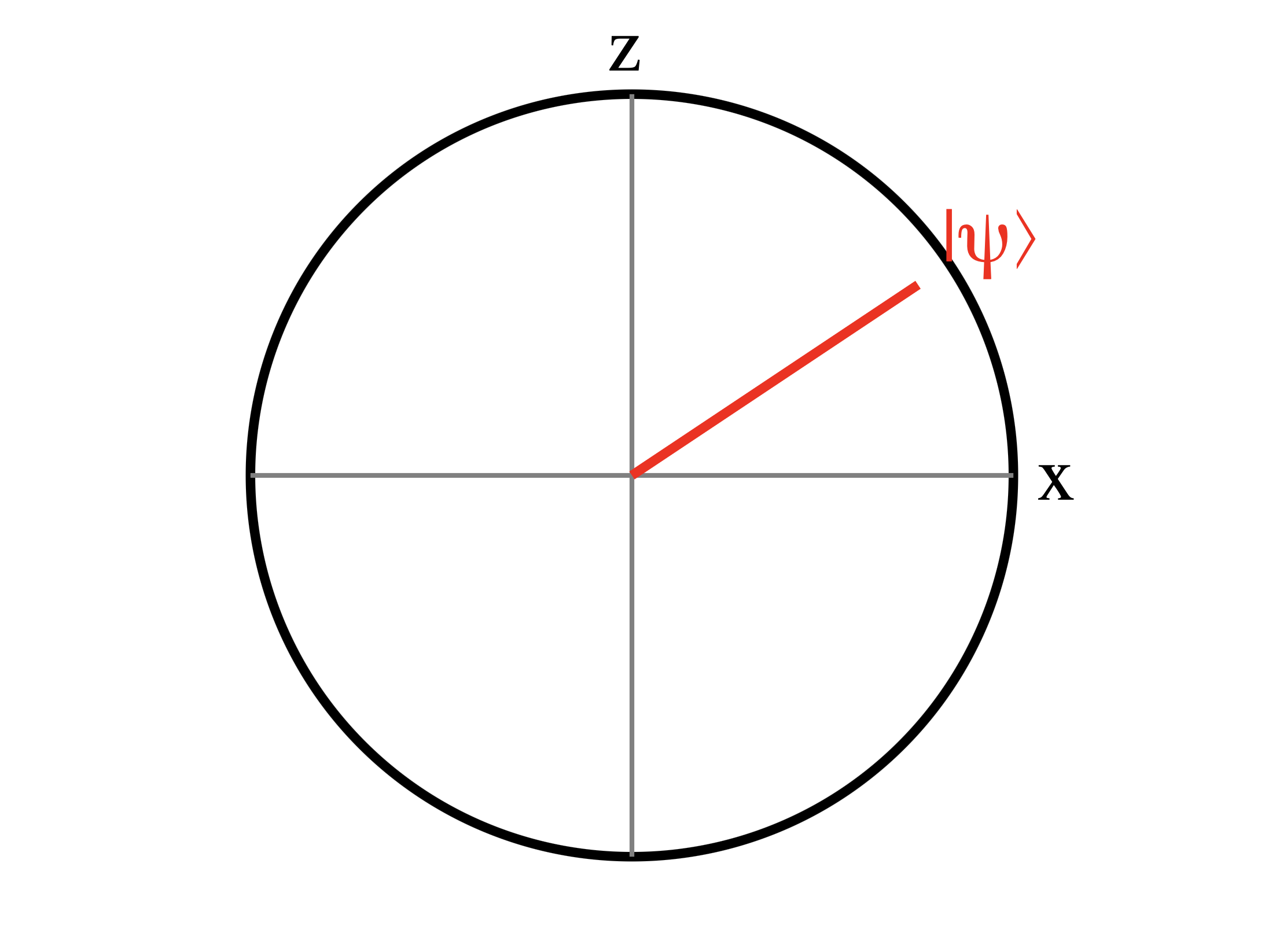
Bloch Sphere for Qubits
For a two-level quantum system (qubit), we can actually visualize the state on a sphere called the Bloch sphere. While this isn’t a general visualization for all quantum states, it’s a useful bridge from classical to quantum thinking. In this representation, the north and south poles might represent the basis states $\vert 0\rangle$ and $\vert 1\rangle$, while any point on the surface represents a superposition of these states.
I also asked my professor about it. He said: “At one point, you don’t actually think about visualising the system. The mathematical framework itself becomes the ‘visualization’ in a sense”.