Machine Learning
Introduction to Machine Learning
We are here:

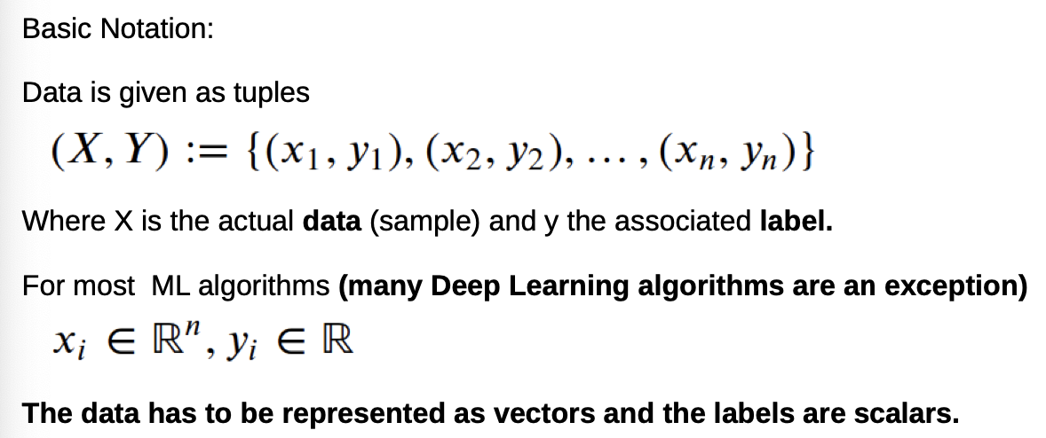
Basic Definitions an Terminology:

Basic Types of ML Algorithms:
- Supervised Learning
- Labeled data
- Direct and quantitative evaluation
- more present, but has limits
- Unsupervised Learning
- Learn models from “ground truth” examples
- Predict unseen examples
- algorithm that we want, but difficult to realize
- Reinforcement Learning
- not that important for us, more present in robotics
Supervised Learning:
General:
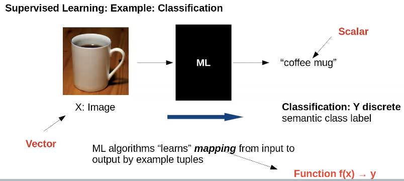
Classification Example:
- Classifications means groupification
- semantic labels are human made (there isn’t a physical law that says what a coffee mug is)→ otherwise, it would be physical modeling, not ML→ semantic labels aren’t 100% accurate, e.g. that could also be a tea mug
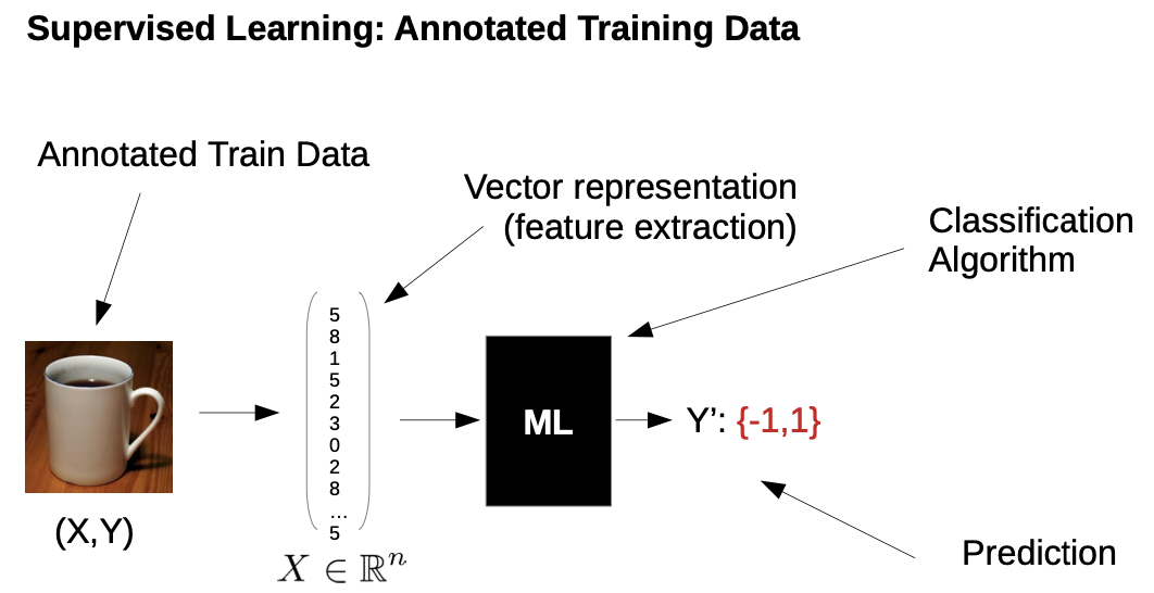
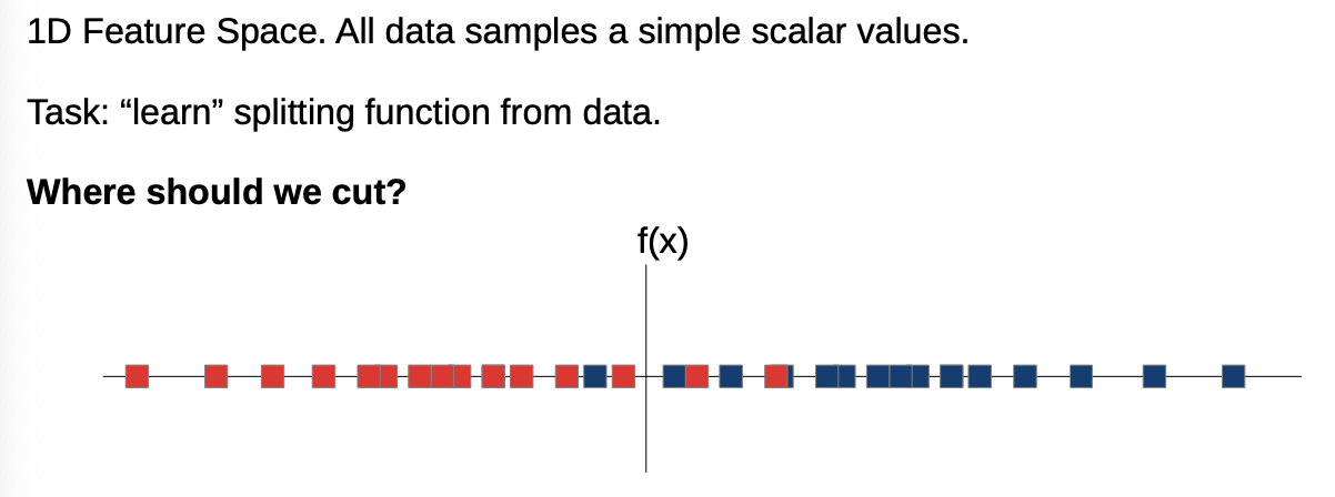
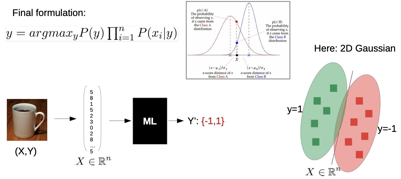
Simple Classification Example: Is it a coffee mug or not?
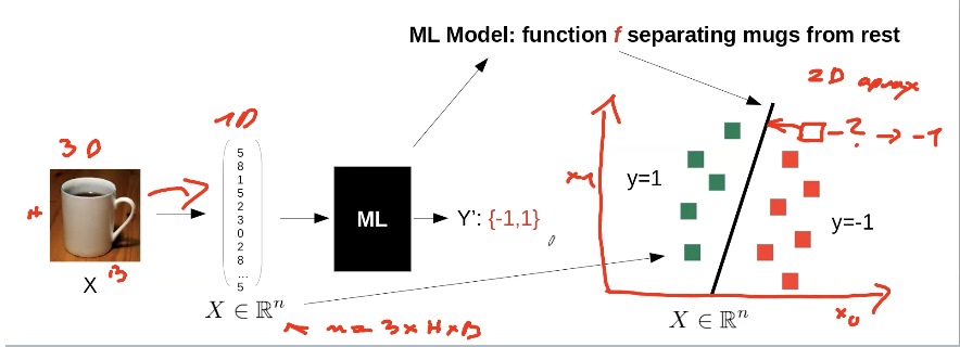
We have a Picture (3D-Tensor), which we convert into a 1D-Vector. Our ML algorithm approximates a function f.
If our 1D-Vector of a picture is on the right side of our function f
→ Y = -1 → no coffee mug
→ Y = 1 → coffee mug
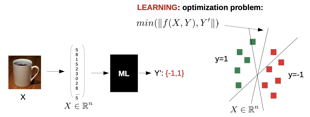
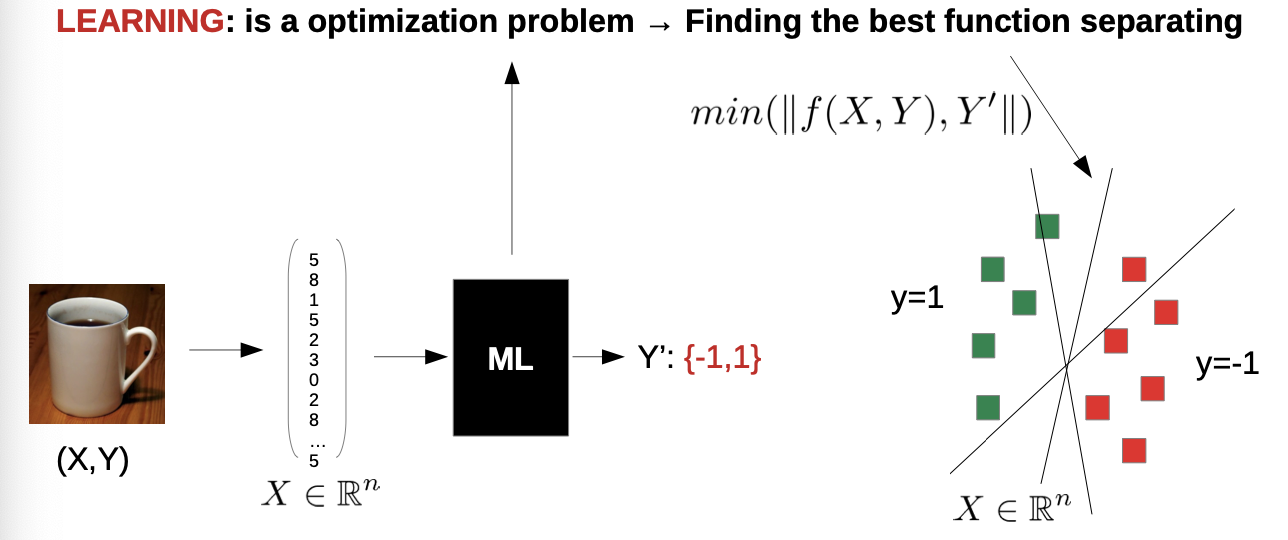
How to find f?
Of a given set of functions, we choose the one which fits the best for our given examples
→ we solve a optimization problem:
(our function is linear, because we have only one classification, coffee mug or not)
Other Example: Regression
→ Predict a next value as accurately as possible
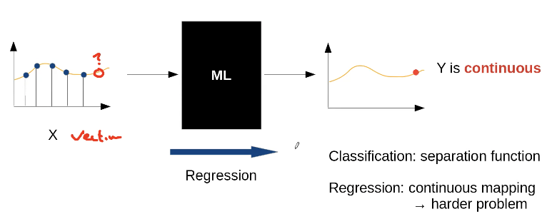
Note: Mathematically, there is nearly no difference between classification and regression
→ you have to decide which type of problem you face
Challenges of Supervised Learning
- need data and Y→ human annotation→ expensive, sometimes impossible to get→ Problem: underfitting
- training data is only a sample, prediction must work on all datae.g. sample: white coffee mug; all data: mugs with different colours→ we want generalization→ Problem: overfitting (Model “too close” to the data, to complex model)
Prevent Overfitting: Data Preparation
Split into train, test data and validate:
- unbiased test set for final evaluation
- hard to guarantee in practice, remember simpson paradox!
- statistical analysis needed
- train set for model training
- validation set (optional, part of train set) can be used to optimize hyper parameters
→ doesn’t actually prevent overfitting, but we can “detect” it
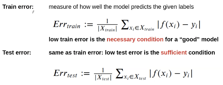
Basic evaluation: (more to come)
Statistics II
Basic Probability Theory

Independence of Events:
Two events are independent when the occurrence of one doesn’t effect the odds other one
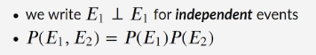
→ multiplication of probabilities if events are independent
Dependence of Events:
Possibilities depends heavily on the given (“secure”) data!
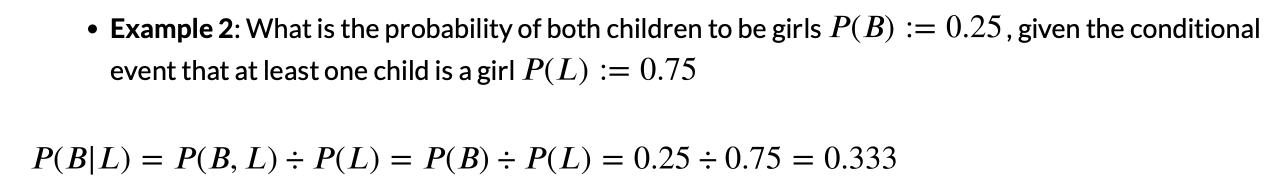
Example: Possibility of giving birth to two girls, when
- when the first baby is already a girl
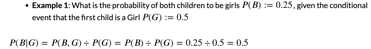
- when at least one child is a girl
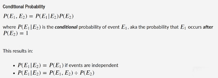
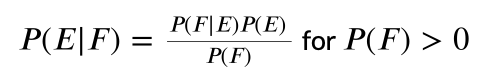
Bayes’ Theorem
→ describes the probability of an event, based on prior knowledge of conditions that might be related to the event
-
we can reverse the deduction of a conditional probability→ we can calculate P(E F) with data from real world that is easier to get - a feature often needed in interference (ML) settings (later more)
Terms:
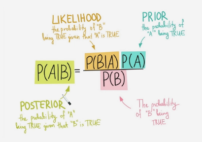
- we can get P(A) and P(B) directly from the data
-
we get P(B A) from our ML models
Example:
We have a drug test that is 99% sensitive and 99% specific. So if a test is positive, the odds says that it’s to 99% likely that the user did take drugs. If a drug test is negative, it’s also to 99% accurate.
Assume that 0.5% of people do take drugs, how are the odds that a random person with a positive drug test is actually positive?

Hypotheses and Statistical Tests
we use statistics and analyze probabilities in order to draw conclusions. A common approach in statistics is to start an experiment with a hypotheses, which is then validated by a statistical test.
Statistical Inference Pipeline
- Formulate Hypotheses
- Design Experiment
- Collect Data
- Test / draw conclusions
Null-Hypotheses:
- The statement being tested in a test of statistical signicance is called the null hypothesis. The test of significance is designed to assess the strength of the evidence against the null hypothesis. Usually, the null hypothesis is a statement of ‘no effect’ or ‘no difference’. It is often symbolized as H(0).
- The statement that is being tested against the null hypothesis is the alternative hypothesis H(1).
- Statistical significance test: Very roughly, the procedure for deciding goes like this: Take a random sample from the population. If the sample data are consistent with the null hypothesis, then do not reject the null hypothesis; if the sample data are inconsistent with the null hypothesis, then reject the null hypothesis and conclude that the alternative hypothesis is true.
Significant Tests:
- p-Value (or significance): is, for a given statistical model, the probability that, when the null hypothesis is true, the statistical test summary would be greater than or equal to the actual observed results.
- at experiment design, a significance threshold alpha is chosen
- typically, alpha=0.05 for scientific experiments
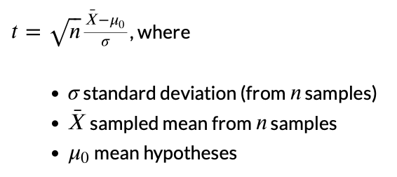
t-Tests
The t-Test (also called Student’s t-Test) compares two averages (means) and tells you if they are different from each other. The t-Test also tells you how significant the differences are; In other words it lets you know if those differences could have happened by chance.
…. many other tests …..
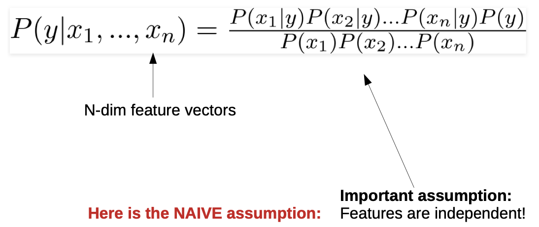
Native Bayes Classifier
Recall from “Introduction to Machine Learning”
How do we evaluate our model?
Example: MNIST Data Base
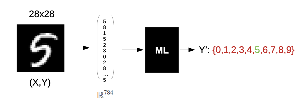
→ A data base with handwritten numbers
Recall: Basic Evaluation
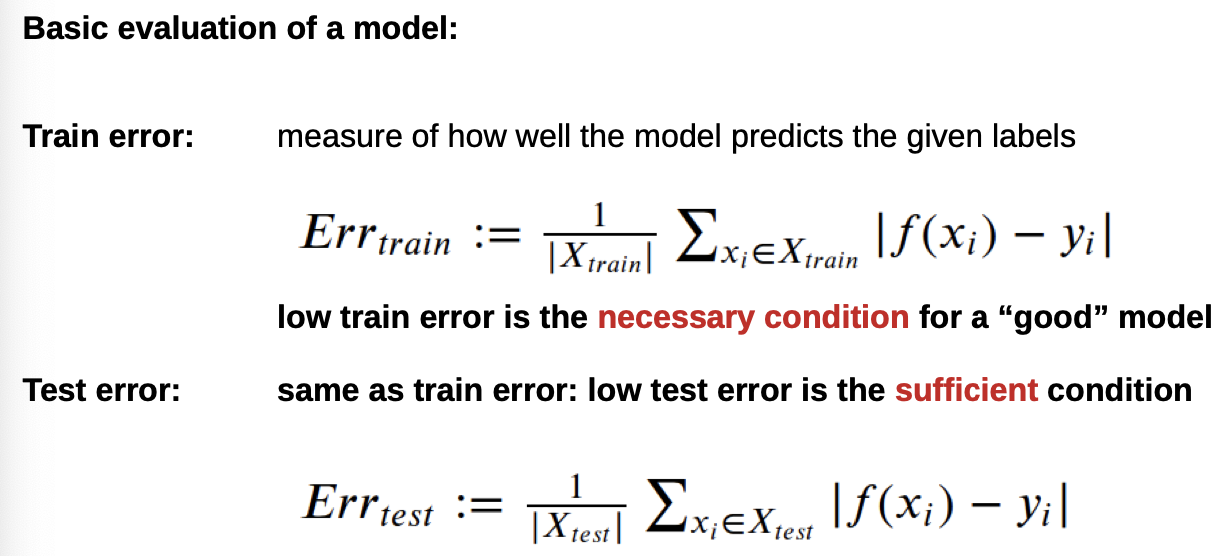
Important:
- For evaluation, use the test set→Otherwise you may get a 100% accuracy for your train set, but it doesn’t work on new data
- if you add the train set, pick numbers randomly→ Otherwise, it could evaluate also the sequence (e.g. 111,222,333,…)
Other Method: Confusion Matrix
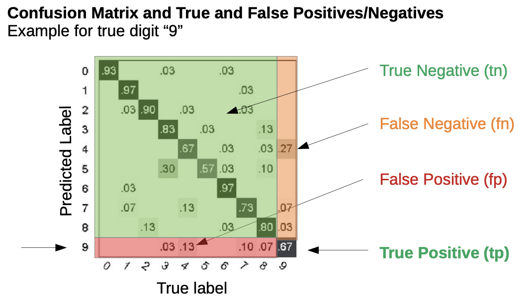
- False Positive: numbers that are incorrectly recognized as a 9
- False Negative: a 9 that isn’t recognized
With this Matrix we can derive quality measures:
- Accuracy is a good measurement as long as all classes have nearly the same occurrencesExtrem negative example: if 90% of the digits are “1”, classifying every digit to “1” will have 90% accuracy!
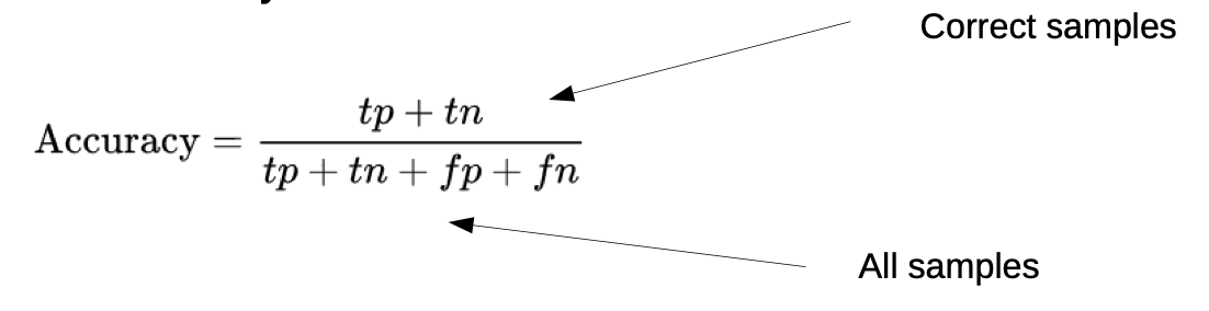
Note: It is a general problem if one event is very unlikely to occur, because many models don’t have enough training data to recognize these events
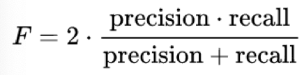
- Precision and Recall
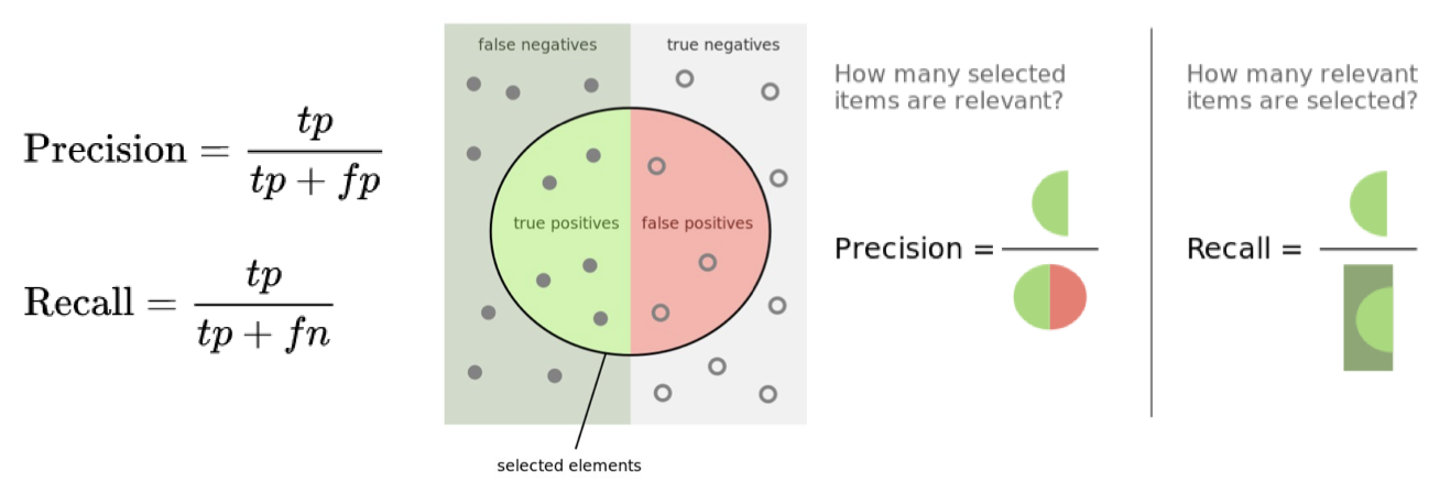
- F-Measure (or balanced F-Score)is the harmonic mean of precision and recall
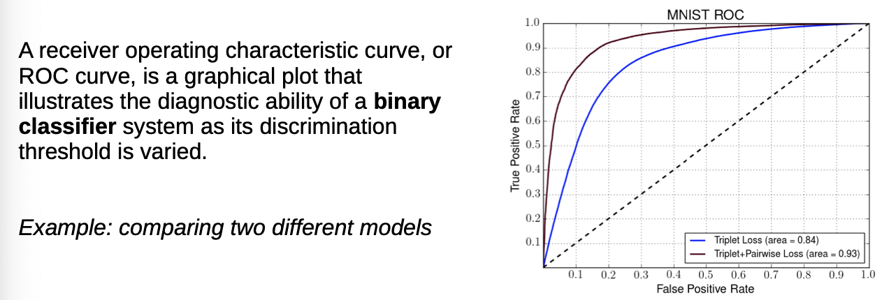
- Receiver Operating Characteristic Curve, area = Integral(→ the higher the area, the better the model)
Simple example:
→ overlapping of data
How do we model that? How do we optimize?
- We can look at the distribution (e.g. Gaussian)
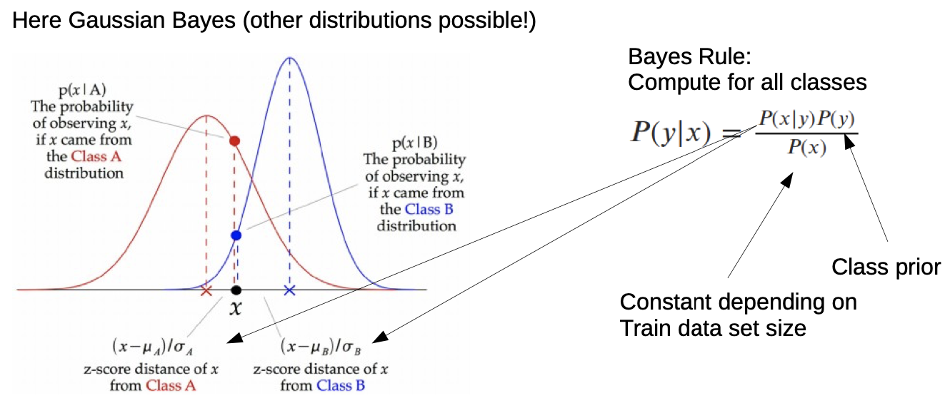
- P (x) is most often constant
→ we can neglect that part
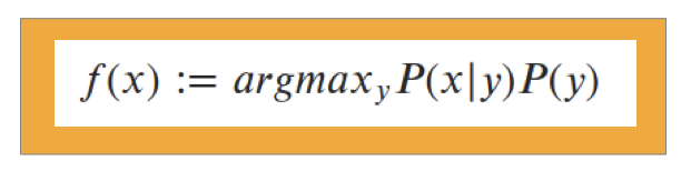
→We calculate which y-value is higher and take that
- depending on the given data, we may have to guess the distribution
- distribution is mostly not Gaussian
- If we have more classes (vectors)
Final notes for Lab Exercise
Good:
- Simple, but powerful model
- doesn’t need much data
- supports complex distributions (like mixture of Gaussians)
- scales well
Bad:
- makes strong assumptions on feature independence
- estimation of complex distributions needs a lot of data
Code Exercises
(Links to Github)
Lab_Matplotlib_Intro_week4.ipynb