SVMs, Model Selection und Outlier Detection
Non-linear Models II
Support Vector Machines
Summary:
- work with small data sets
- for classification and regression
- gives us the “one” best solution
- non-linear → many possibilities
- can be computing intensive with many classes, large data sets
Basic model
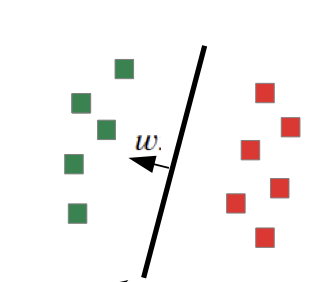
- Linear classification
- Support only two classes {-1, 1}
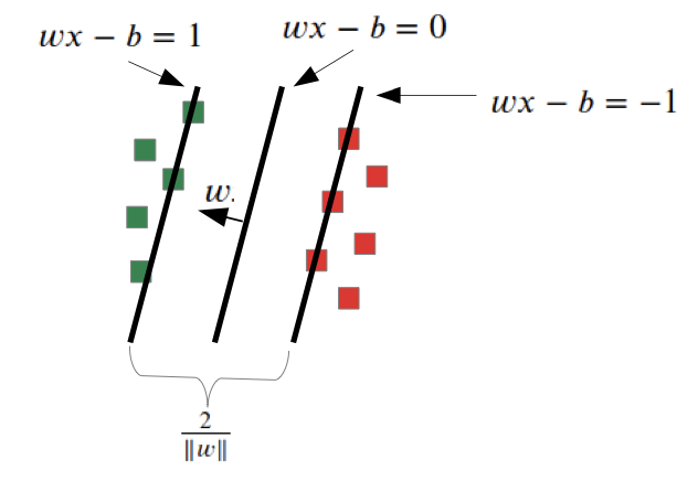
- Parametrization: $wx - b = 0$ (w is orthogonal to the line)
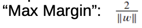
New optimization problem: “Max Margin”
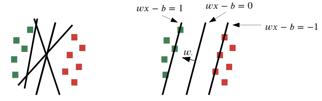
With our previous optimization problem (Loss function), we could get many different solution depending on e.g. step size.
With an additional optimization problem (Max Margin), we search for the solution with the highest gap between the data sets and our function.
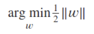
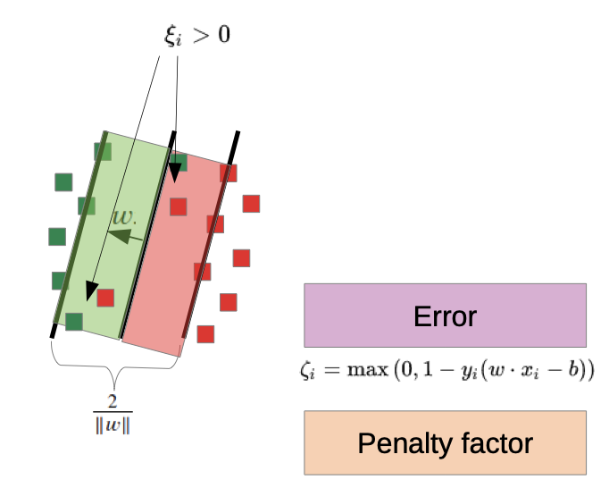
Subject to (Nebenbedingung):
→ one solution, always the best solution
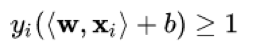
Soft Margin: allow some outliers
- we allow outliers, but we “punish” them
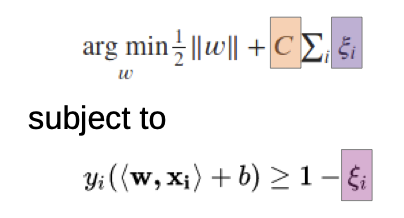
- only for the outliers is $\xi_i \neq 0$
- C is the penalty factor, higher C value punishes outliers more
The minimization problem is not easy to solve, so we use a Dual Formulation
Dual formulation of the optimization problem
(we don’t derive it in our lectures, but this is the common approach)
we re-parameterize the w
→ we rewrite the w as a linear combination of samples
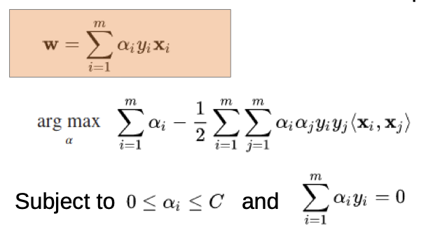
- $x^{(i)}$, $x^{(j)}$ are our data sets
- $y^{(i)}$, $y^{(j)}$ are our different outcomes
- alpha is our weighting (with we optimize for), alphas are “pushing” from both sides to the line, we search a balance
- C is our penalty factor
→ Dual formulation via Lagrange dual function
→ Converts our optimization problem from minimization to maximization
Classification
Suppose we have trained our model (we know all the $\alpha^{(i)}$)
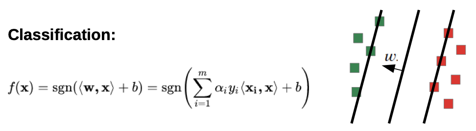
If we want to classify a point x, we have to build the scalar product with all the other points with their weighting.
→ we have to calculate all the scalar products for every new evaluation
→ large number of computations
BUT: only a few vectors have $\alpha \neq 0$
(only the points that lay on the margin or in the soft margin)
→ we only have to remember these vectors, they are called support vectors
Non-Linear SVMs
→ follow same strategy as before and add simple non-linear function
At the formulation of the model normal:
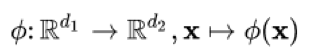
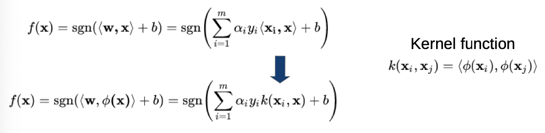
- scalar product is replaced by a kernel function
- kernel function is the scalar product of two values with are transformed by the non-linear function phi
- don’t have to be element-wise (like previously), can also be vector-wise
Typical kernel functions:
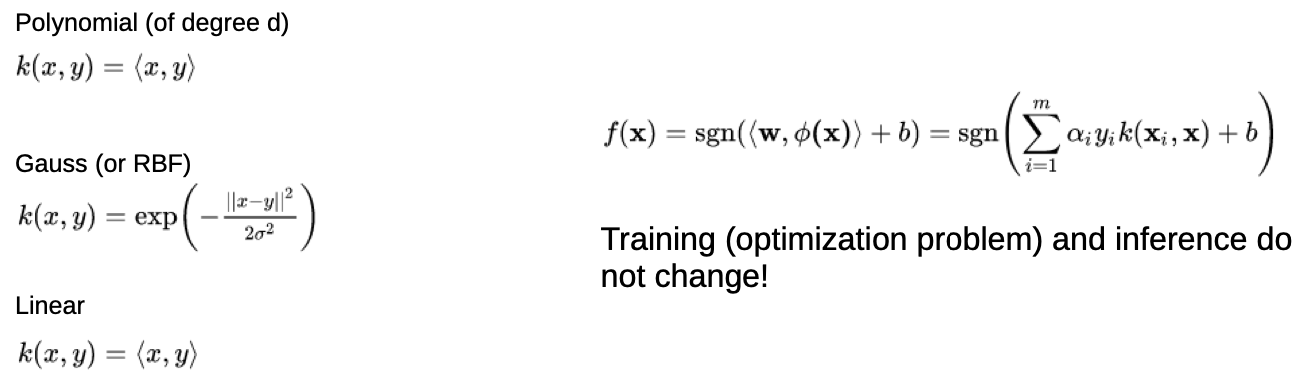
Multi class problems:
1-vs-rest approach
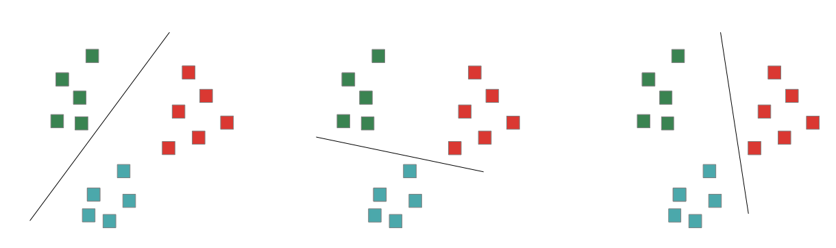
Train N models, take which solution fits the best
1-vs-1 approach
N(N-1)/2 models in a tree execution, take best
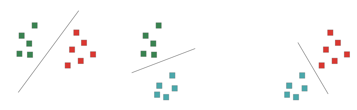
→ in real Projects, this is only a Parameter (1-vs-1 or 1-vs-rest), it happens under the hood
Code Exercises
(Links to Github)